DP Scree Plots • dppca

This tutorial shows how to use dp_scree() to estimate private scree values and proportions of variance explained (PVE), inspect the results, and draw scree and PVE plots. Also, it explains how to choose among the clipped mean, private modified winsorized mean (PMWM), and Huber mean estimators.

The focus here is on R arguments, control settings, and visualization. For the paired-difference construction, mathematical formulas, and privacy accounting, see DP Scree Methodology. For installation, example datasets, input requirements, and general privacy budget allocation, see Getting Started.

1. Load the example data

We use gau, a synthetic dataset with 1,000 observations and 20 numeric variables. For more details, see the documentation for gau.

library(dppca)
data("gau", package = "dppca")

X <- gau
dim(X)
#> [1] 1000   20

2. Set the privacy budget and estimate scree values

Scree estimation needs a loading budget for private PC directions and a scree budget for the private variance estimator. When split is omitted,dp_scree() divides the total budget equally between these two components.

scree_privacy <- privacy_control(
  eps = 6,
  delta = 1e-4
)

You can also specify a different allocation using split as explained in Getting Started.

First, we use the clipped mean method to estimate scree values for the first five PCs:

set.seed(123)
scree_fit <- dp_scree(
  X,
  k = 5,
  privacy = scree_privacy,
  method = "clipped",
  control = clipped_control(C_clip = 20),
  non_private = TRUE
)

scree_fit
#> Differentially Private Scree Estimates
#> Data: 1000 observations x 20 variables
#> Components: 20 PC directions; 5 scree estimates
#> Methods: scree = clipped 
#> Total privacy budget: eps = 6; delta = 1e-04
#> Non-private reference: included

The clipped_control() function requires a public clipping threshold. The value C_clip = 20 is an illustrative setting, not an automatic or universally recommended choice.

The main arguments of dp_scree() are:

Argument	Description
`X`	Input observations, with numeric features in columns.
`k`	Number of leading PCs to estimate, from 1 to the number of numeric variables.
`privacy`	Total budget and loading/scree allocation from `privacy_control()`.
`method`	One or more of `"clipped"`, `"pmwm"`, and `"huber"` (default: `"clipped"`).
`control`	Method-specific tuning parameters, specified using `clipped_control()`, `pmwm_control()`, or `huber_control()`.
`cpp.option`	Use the compiled direction estimator (`TRUE`, the default) or its R implementation (`FALSE`).
`mono`	Enforce a nonincreasing scree sequence via isotonic regression (default: `TRUE`).
`non_private`	Compute an ordinary PCA comparison when `TRUE` (default: `FALSE`).
`V_dp`	Optionally reuse previously estimated private directions; their earlier loading budget must still be recorded.

3. Inspect and plot the result

Printing scree_fit shows a short overview of the fitted results. To see scree values, PVE, and cumulative PVE for each stored method, use summary():

scree_summary <- summary(scree_fit)
scree_summary
#> DP Scree Estimates Summary
#> Data: 1000 observations x 20 variables
#> Components: 20 PC directions; 5 scree estimates
#> Methods: scree = clipped 
#> 
#> DP component importance:
#>                    PC1    PC2    PC3    PC4    PC5
#> Eigenvalue     12.0624 7.4371 3.9225 3.9225 3.9225
#> PVE             0.3858 0.2379 0.1255 0.1255 0.1255
#> Cumulative PVE  0.3858 0.6236 0.7491 0.8745 1.0000
#> 
#> Proportions are normalized over 5 estimated components.
#> 
#> Allocated privacy budget:
#>         eps delta
#> Loading   3 5e-05
#> Scree     3 5e-05
#> Total     6 1e-04
#> 
#> Non-private reference: included

The numeric estimates remain directly accessible by method. The optional ordinary PCA reference is under nonprivate, while data dimensions, selected methods, and privacy allocations are under metadata:

scree_fit$clipped$scree
#>       PC1       PC2       PC3       PC4       PC5 
#> 12.062398  7.437085  3.922463  3.922463  3.922463
scree_fit$clipped$pve
#>       PC1       PC2       PC3       PC4       PC5 
#> 0.3857885 0.2378583 0.1254511 0.1254511 0.1254511
scree_fit$nonprivate$scree
#>       PC1       PC2       PC3       PC4       PC5 
#> 37.312574 12.616374  5.206048  5.075826  4.850032
scree_fit$metadata$privacy
#> $total
#>   eps delta 
#> 6e+00 1e-04 
#> 
#> $budgets
#> $budgets$loading
#>   eps delta 
#> 3e+00 5e-05 
#> 
#> $budgets$scree
#>   eps delta 
#> 3e+00 5e-05 
#> 
#> 
#> attr(,"class")
#> [1] "dppca_privacy_control"

In a default private-only fit (non_private = FALSE), scree_fit$nonprivate is NULL; scree_fit$clipped, $pmwm, or $huber remain top-level method results.

By default, plot() displays both the PVE and scree plots side by side. Because this example was fitted with non_private = TRUE, the ordinary PCA reference is included automatically; a fit with non_private = FALSE shows only private estimates:

plot(scree_fit)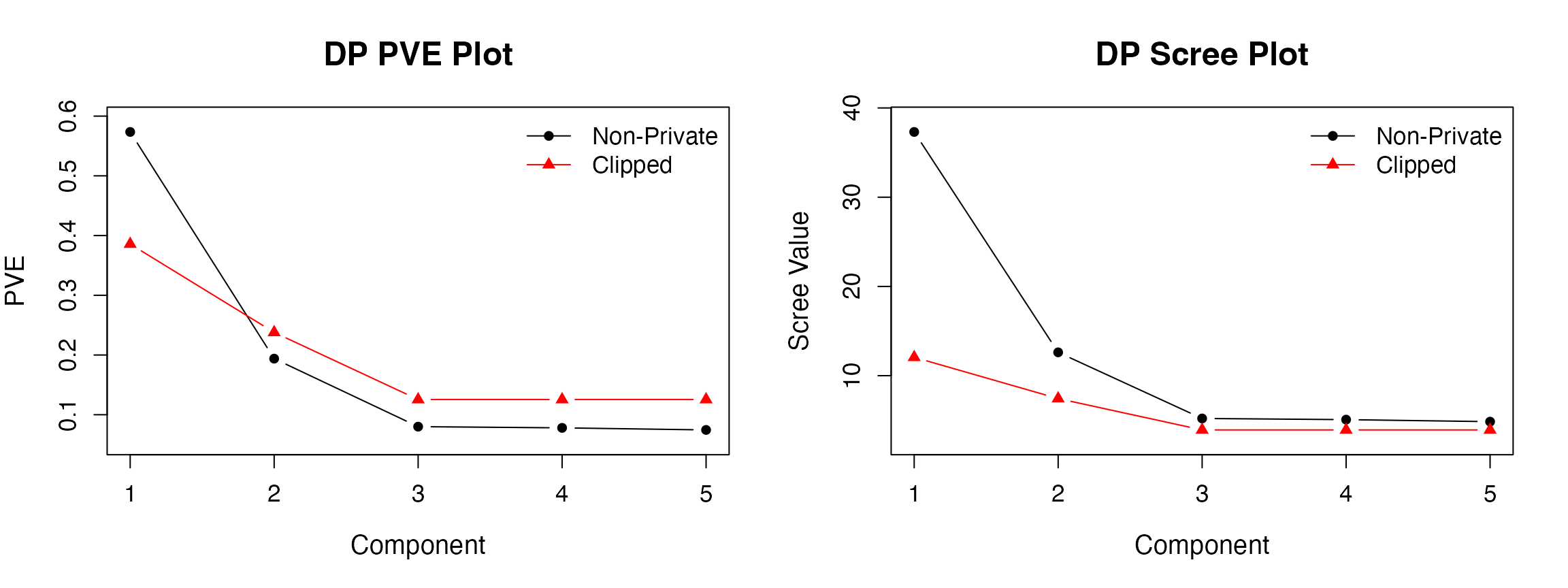

Private and ordinary PCA PVE and scree plots

To display only one view, use type.

plot(scree_fit, type = "pve")
plot(scree_fit, type = "scree")

Plot type	What it shows
`"pve"`	Each component’s share of the estimated variation among the `k` fitted PCs.
`"scree"`	Estimated variation along each private PC direction, on its original scale.

4. Choose a method and its tuning parameters

The three scree estimators use the same projected paired differences, but differ in how they estimate their means. The tables below map the symbols used in DP Scree Methodology** to the R arguments of each method-specific control function.

Clipped mean

Clipped estimation limits each squared pair difference before releasing a noisy mean. See Clipped Mean Methodology.

Theory notation	R argument	Meaning
C_{\mathrm{clip}}	`C_clip`	Positive upper clipping threshold; controls the bias–noise tradeoff (required, no default).

The setting used in Section 2 is:

clipped_set <- clipped_control(C_clip = 20)
clipped_set
#> $C_clip
#> [1] 20

A smaller C_clip reduces sensitivity and Gaussian noise, but can truncate more large paired differences. A larger value reduces clipping bias while requiring more privacy noise.

Private modified winsorized mean (PMWM)

PMWM privately estimates lower and upper cutoffs and then computes a noisy winsorized mean. See PMWM Methodology.

Theory notation	R argument	Meaning
a,b	`a`, `b`	Public lower and upper bounds for the estimated cutoffs, with a<b (required).
c_{\mathrm{trim}}	`trim_const`	Positive baseline trimming constant in the quantile level (required).
\eta_{\mathrm{trim}}	`eta`	Lower-bound tuning value for the trimming proportion, in [0,0.5) (required).
\beta	`beta`	Geometric quantile-search grid base, greater than 1 (default: `1.001`).
I_Q,I_M	`split_mode`	`FALSE`: reuse all pair rows in both stages (default); `TRUE`: use disjoint quantile and mean subsets.

For example, to use PMWM instead of the clipped estimator:

pmwm_set <- pmwm_control(
  a = 0,
  b = 50,
  trim_const = 10,
  eta = 0.01
)

set.seed(123)
pmwm_fit <- dp_scree(
  X,
  k = 5,
  privacy = scree_privacy,
  method = "pmwm",
  control = pmwm_set,
  non_private = TRUE
)

summary(pmwm_fit)
plot(pmwm_fit, type = "pve")

Huber mean

The Huber method privately estimates a scale for each PC and uses thatscale to set a Huber threshold for noisy gradient descent. See Huber Mean Methodology.

Theory notation	R argument	Meaning
r_{\min},r_{\max}	`k_min_m2`, `k_max_m2`	Integer limits for the dyadic scale candidates 2^r, with r_{\min}<r_{\max} (required).
\rho	`m2_frac`	Fraction of scree epsilon used for private scale estimation, in (0,1) (required).
\mu_0	`mu0`	Public initial mean iterate (default: `0`).
\eta_0	`eta0`	Positive gradient-descent step size (default: `1`).
T	`T`	Number of noisy gradient steps (default: `ceiling(log(m))`).
M	`M`	Number of blocks for private scale estimation (default: `floor(sqrt(m / 2))`, capped by available pairs).

When T or M is left as NULL, the corresponding sample-size-based default is used.

For example:

huber_set <- huber_control(
  k_min_m2 = -10,
  k_max_m2 = 10,
  m2_frac = 0.25
)

set.seed(123)
huber_fit <- dp_scree(
  X,
  k = 5,
  privacy = scree_privacy,
  method = "huber",
  control = huber_set,
  non_private = TRUE
)

summary(huber_fit)
plot(huber_fit, type = "pve")

5. Compare multiple methods and account for releases

To fit several methods using one private direction estimate, provide a vector of method names and a named list of their corresponding controls:

set.seed(123)
scree_comparison <- dp_scree(
  X,
  k = 5,
  privacy = scree_privacy,
  method = c("clipped", "pmwm", "huber"),
  control = list(
    clipped = clipped_set,
    pmwm = pmwm_set,
    huber = huber_set
  ),
  non_private = TRUE
)

summary(scree_comparison)
#> DP Scree Estimates Summary
#> Data: 1000 observations x 20 variables
#> Components: 20 PC directions; 5 scree estimates
#> Methods: scree = clipped, pmwm, huber 
#> 
#> DP component importance (clipped):
#>                    PC1    PC2    PC3    PC4    PC5
#> Eigenvalue     12.0624 7.4371 3.9225 3.9225 3.9225
#> PVE             0.3858 0.2379 0.1255 0.1255 0.1255
#> Cumulative PVE  0.3858 0.6236 0.7491 0.8745 1.0000
#> 
#> DP component importance (pmwm):
#>                    PC1    PC2     PC3     PC4     PC5
#> Eigenvalue     22.6834 8.5897 2.80526 2.80526 2.80526
#> PVE             0.5715 0.2164 0.07068 0.07068 0.07068
#> Cumulative PVE  0.5715 0.7880 0.85864 0.92932 1.00000
#> 
#> DP component importance (huber):
#>                    PC1     PC2     PC3     PC4     PC5
#> Eigenvalue     18.5145 2.22032 2.22032 2.22032 2.22032
#> PVE             0.6758 0.08105 0.08105 0.08105 0.08105
#> Cumulative PVE  0.6758 0.75686 0.83791 0.91895 1.00000
#> 
#> Proportions are normalized over 5 estimated components.
#> 
#> Allocated privacy budget (per method):
#>         eps delta
#> Loading   3 5e-05
#> Scree     3 5e-05
#> Total     6 1e-04
#> 
#> All scree methods use the same privately estimated PC directions.
#> 
#> Non-private reference: included

plot(scree_comparison, type = "pve")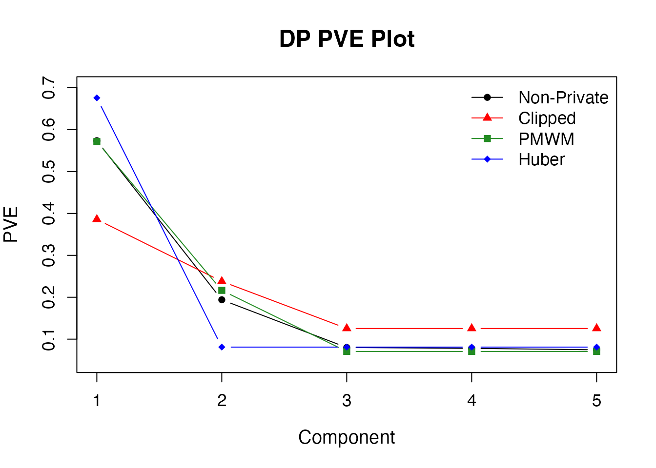

PVE comparison of clipped, PMWM, Huber, and ordinary PCA

Within a call, all methods share a single private direction estimate but independently compute their scree estimates using the full scree privacy budget.

6. Reusing Private PC Directions

When supplying previously estimated directions through V_dp, specify the actual privacy budget used to estimate those directions as the loading allocation. This records the previously incurred privacy cost without spending the loading budget again.

There are two ways to specify the privacy allocation.

Option 1: Specify component budgets directly.

# Estimate private PC directions.
loading_fit <- dp_loading(
  X,
  eps = 3,
  delta = 5e-5
)

# Specify the actual loading budget and the scree budget.
reuse_privacy <- privacy_control(
  loading = c(eps = 3, delta = 5e-5),
  scree   = c(eps = 3, delta = 5e-5)
)

Option 2: Specify a total budget and allocation proportions.

reuse_privacy <- privacy_control(
  eps = 6,
  delta = 1e-4,
  split = c(loading = 0.5, scree = 0.5)
)

# Estimate private PC directions using the allocated loading budget.
loading_budget <- reuse_privacy$components$loading

loading_fit <- dp_loading(
  X,
  eps = loading_budget[["eps"]],
  delta = loading_budget[["delta"]]
)

After either option, the estimated directions can be reused in dp_scree():

scree_reused <- dp_scree(
  X,
  k = 5,
  privacy = reuse_privacy,
  method = "clipped",
  control = clipped_control(C_clip = 20),
  V_dp = loading_fit$directions,
  non_private = FALSE
)

summary(scree_reused)

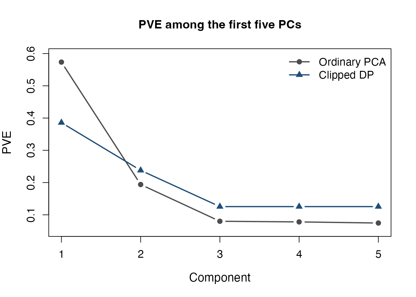
7. Customize the plot

Use scree_plot_control() to change the appearance of the stored plot.

plot(
  scree_fit,
  type = "pve",
  plot_control = scree_plot_control(
    title = "PVE among the first five PCs",
    col = c(nonprivate = "grey30", clipped = "#1F4E79"),
    legend_labels = c(nonprivate = "Ordinary PCA", clipped = "Clipped DP"),
    lwd = 2,
    point_cex = 1.2,
    cex_main = 1.2,
    legend_position = "topright"
  )
)

Customized PVE plot comparing private and ordinary PCA

Setting	What it changes
`title`, `xlab`, `ylab`	Plot title and axis labels.
`col`, `lty`, `pch`	Named series colors, line types, and point symbols.
`lwd`, `point_cex`	Line width and point-size multiplier.
`cex_main`, `cex_lab`, `cex_axis`	Title, axis-label, and tick-label sizes.
`legend_position`, `legend_labels`, `cex_legend`, `legend_bty`	Legend position, labels, size, and border.

For complete argument descriptions, see ?dp_scree, ?plot.dp_scree, and ?scree_plot_control.

Previous: DP Loading Plot
Next: DP Score Plot
Tutorial overview: Choose a starting point