DP Score Plots

This tutorial shows how to use dp_score() to estimate private 2D score histograms, inspect their stored probabilities, and display them as histograms or synthetic score points. It also covers the additive and sparse estimators, grouped plots, plot controls, and reuse of previously estimated private PC directions.

The focus is on R arguments, examples, and visualization. For the mathematics of the private frame, histogram mechanisms, and privacy accounting, see DP Score Methodology. For data requirements and general budget allocation, see Getting Started.

1. Load the example data

We use gau, a synthetic dataset containing 1,000 observations and 20 numeric variables. For dataset details, see the gau.

library(dppca)
data("gau", package = "dppca")

X <- gau
dim(X)
#> [1] 1000   20

2. Set the privacy budget and estimate a score histogram

A dp_score() fit needs two privacy components: loading, to estimate private PC directions, and score, to estimate the private plotting frame and the histogram. If split is omitted, dp_score() allocates the total privacy budget equally between them.

score_privacy <- privacy_control(
  eps = 6,
  delta = 1e-4
)

In this example, loading and score each receive (\varepsilon,\delta)=(3,5\times10^{-5}) when used by dp_score(). Within the score allocation, the package automatically assigns 35% of score epsilon to frame estimation, 65% to the histogram, and all score delta to the histogram.

First, we use both the additive and sparse histogram methods, without retaining non-private reference data:

set.seed(123)
score_fit <- dp_score(
  X,
  privacy = score_privacy,
  bins = c(10, 10),
  method = c("add", "sparse"),
  axes = c(1, 2),
  non_private = FALSE
)

score_fit
#> Differentially Private Score Histograms
#> Data: 1000 observations x 20 variables
#> Score axes: PC1, PC2 
#> Grid: 10 x 10 
#> Methods: score = add, sparse 
#> Total privacy budget (per histogram method): eps = 6; delta = 1e-04
#> Non-private reference: not stored

The main arguments of dp_score() are:

Argument	Description
X	Input observations; numeric features in columns. The selected group column, if any, is excluded from PCA.
privacy	Loading/score allocations from privacy_control(); an omitted split gives an equal two-way allocation for dp_score().
bins	Positive integer vector c(m_x, m_y) specifying the numbers of horizontal and vertical histogram bins (required).
method	One or both of "add" (Gaussian) and "sparse" (stability-based); default: c("add", "sparse").
axes	Two distinct PC indices, in horizontal/vertical order (default: c(1, 2)).
cpp.option	Use the compiled direction estimator (TRUE, the default), or the R implementation (FALSE).
V_dp	Reuse a previously estimated full private direction matrix; the loading allocation must record its actual prior privacy cost.
non_private	Retain ordinary PCA reference scores and histograms when TRUE (default: FALSE).
group	A group-column name or a label vector; NULL (default) fits a pooled histogram. Groups must be publicly fixed for the stated parallel-composition argument.

The V_dp argument allows previously estimated private PC directions to be reused in dp_score(). For a detailed example, see Reusing Private PC Directions in the DP Scree Plot tutorial.

2.1. Additive and sparse methods

The two estimators differ in how they perturb bin frequencies. The full mathematical definitions are in Additive histogram and Sparse histogram.

Method	What to expect
"add"	Adds Gaussian noise to every count; normalizes truncated positive counts.
"sparse"	Adds Laplace noise only to nonempty bin proportions; keeps cells passing a threshold and may produce an all-zero histogram.

3. Inspect and plot the result

3.1. Read the fit and stored estimates

Printing the fitted object gives a summary of the stored results. summary() reports the frame, grid, grouping information when applicable, and positive bin counts and probability sums:

score_summary <- summary(score_fit)
score_summary
#> DP Score Histograms Summary
#> Data: 1000 observations x 20 variables
#> Score axes: PC1, PC2 
#> Grid: 10 x 10 
#> Methods: score = add, sparse 
#> 
#> Private frame:
#>  Axis  Center  Lower Upper
#>   PC1 0.05101 -15.68 15.78
#>   PC2 0.14947 -15.58 15.88
#> 
#> Histogram summary:
#>  Method Bins Positive bins Probability sum
#>     add  100            66               1
#>  sparse  100            20               1
#> 
#> Allocated privacy budget (per histogram method):
#>                  eps delta
#> Loading         3.00 5e-05
#> Score frame     1.05 0e+00
#> Score histogram 1.95 5e-05
#> Total           6.00 1e-04
#> 
#> All histogram methods use the same private PC directions and frame.
#> 
#> Non-private reference: not stored

You can inspect the same results directly:

score_fit$frame
#> $xlim
#> [1] -15.67937  15.78139
#> 
#> $ylim
#> [1] -15.58090  15.87985
head(score_fit$add)
#>           xmin         xmax     ymin      ymax         prob
#> 1 -15.67936864 -12.53329290 -15.5809 -12.43483 0.0000000000
#> 2 -12.53329290  -9.38721716 -15.5809 -12.43483 0.0021982799
#> 3  -9.38721716  -6.24114142 -15.5809 -12.43483 0.0003693919
#> 4  -6.24114142  -3.09506569 -15.5809 -12.43483 0.0022237447
#> 5  -3.09506569   0.05101005 -15.5809 -12.43483 0.0000000000
#> 6   0.05101005   3.19708579 -15.5809 -12.43483 0.0026362709
sum(score_fit$add$prob)
#> [1] 1
score_fit$metadata$method
#> [1] "add"    "sparse"
score_fit$metadata$privacy
#> $total
#>   eps delta 
#> 6e+00 1e-04 
#> 
#> $budgets
#> $budgets$loading
#>   eps delta 
#> 3e+00 5e-05 
#> 
#> $budgets$score
#>   eps delta 
#> 3e+00 5e-05 
#> 
#> 
#> attr(,"class")
#> [1] "dppca_privacy_control"

Stored component	Meaning
score_fit$frame$xlim, $ylim	Private horizontal and vertical plotting limits.
score_fit$add	Data frame with xmin, xmax, ymin, ymax, and prob for every cell.
score_fit$add$prob	Estimated probability mass in each cell, not density height or an observed cell count.
score_fit$nonprivate	NULL here (non_private = FALSE); when requested, stores ordinary PCA reference results.
score_fit$nonprivate$scores	Centered ordinary PCA score coordinates, available only when non_private = TRUE.
score_fit$nonprivate$frame, $histogram	Ordinary reference frame and histogram when requested.
score_fit$metadata	Data dimensions, axes, bin counts, method(s), privacy allocation, and grouping settings.

3.2. Show a private histogram

histogram_plot <- plot(
  score_fit,
  type = "histogram"
)

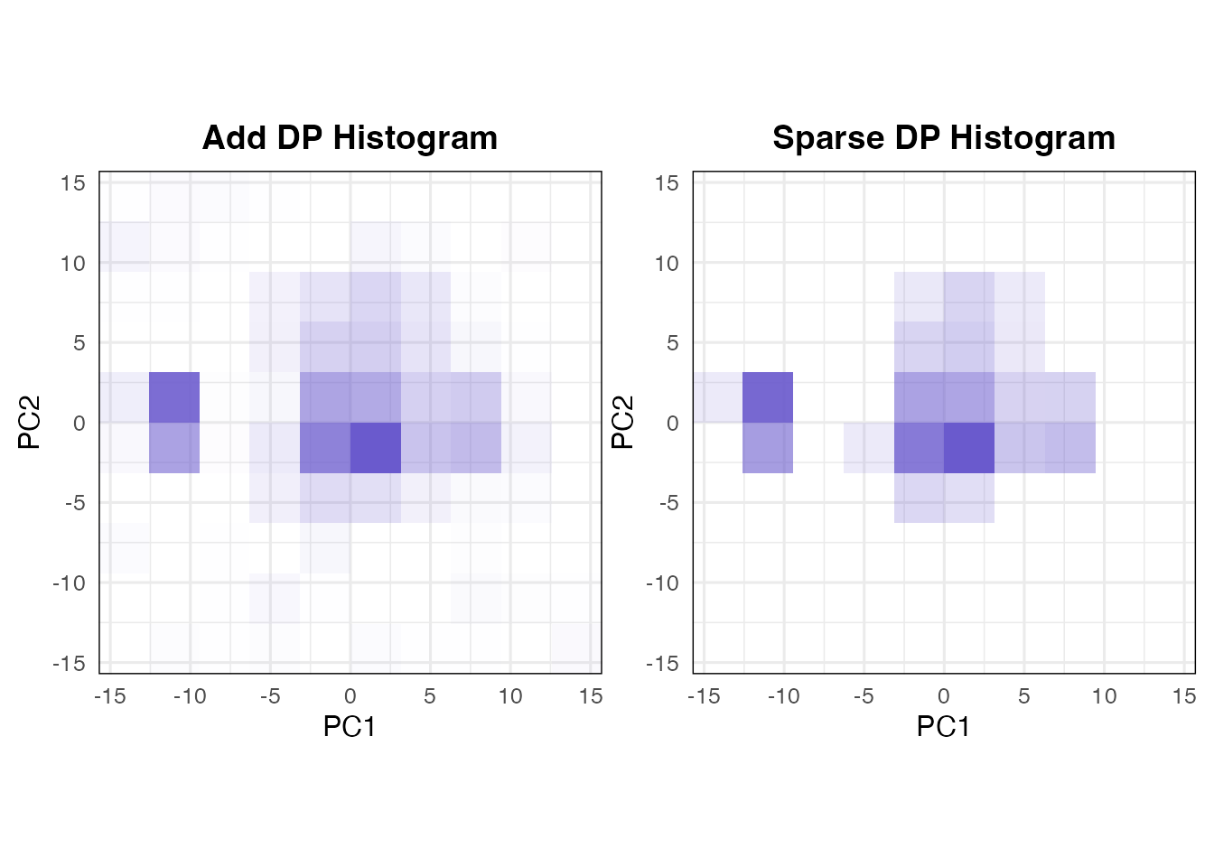
The shade of a cell represents its estimated probability mass.

The center argument controls display centering, not the estimation of private directions, the score frame, or histogram probabilities. By default, center = TRUE shifts the midpoint of the privately estimated score frame to (0,0) in both histogram and synthetic-sample plots, See Display centering.

To retain the original private frame coordinates in the plots, set center = FALSE explicitly:

set.seed(321)
plot(score_fit, type = c("histogram", "sample"), center = FALSE)

3.3. Draw synthetic score points

The same fitted histogram can be displayed as synthetic points.

set.seed(321)
sample_plot <- plot(
  score_fit,
  type = "sample",
  sampling_control = sampling_control(
    method = "uniform",
    sample_size = 500,
    bandwidth_scale = 0.1
  )
)

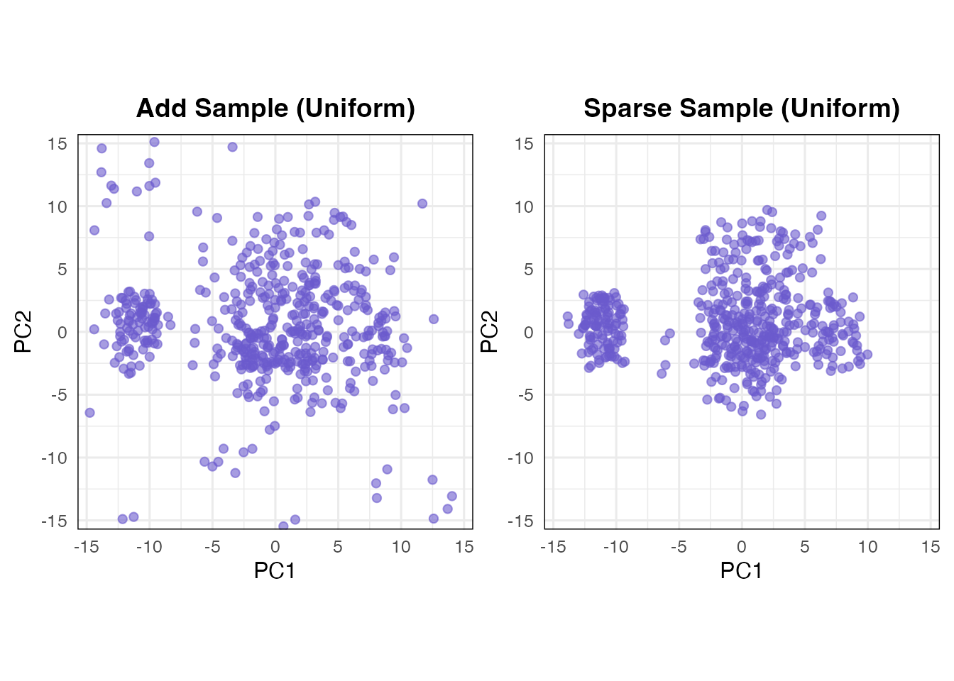
These are 500 newly generated coordinates. A bin is first selected using the stored private probabilities; the point is then generated within that bin or at its center, optionally with Gaussian jitter. See Synthetic score sampling.

The main arguments of sampling_control() are:

Setting	Description
method = "uniform"	Draw uniformly inside a sampled bin, followed by optional jitter (default).
method = "center"	Start at a sampled bin’s center, followed by optional jitter.
sample_size = NULL	By default, generate the same number of synthetic points as the original observations (1,000 in this example).
bandwidth_scale = NULL	Use method-specific default jitter multipliers: center = 0.5 and uniform = 0.25.
bandwidth_scale = 0	Disable jitter; "center" then produces points exactly at bin centers.

When dp_score() is fitted with non_private = TRUE, plot() automatically includes non-private comparison panels. For sample plots, the non-private panel displays the original centered PCA scores by default, while the private panel displays synthetic points generated from the DP histogram. If sample_size is explicitly specified, both panels display the specified number of synthetic points sampled from their respective histograms. A fit with non_private = FALSE displays only private panels; plot() has no separate non_private option.

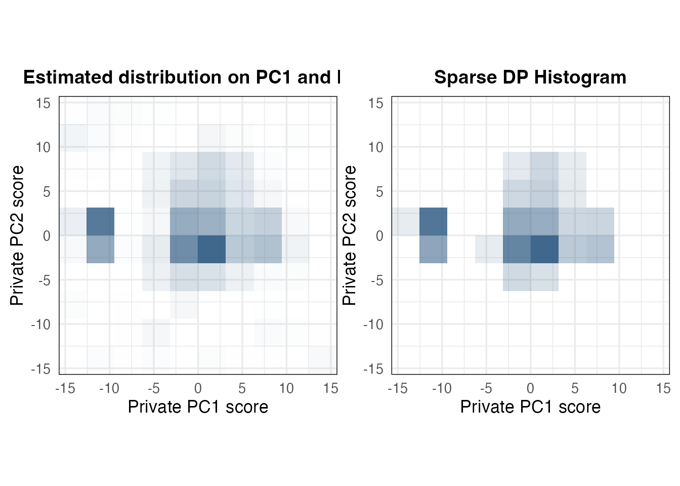
4. Customize the plot

Use score_plot_control() to adjust colors, labels, point sizes, and the group legend.

plot(
  score_fit,
  type = "histogram",
  plot_control = score_plot_control(
    color = "#1F4E79",
    add_title = "Estimated distribution on PC1 and PC2",
    xlab = "Private PC1 score",
    ylab = "Private PC2 score",
    hist_alpha_range = c(0, 0.85),
    base_size = 13,
    title_size = 14
  )
)

Plot setting	What it changes
color, hist_alpha_range	Default histogram/scatter color and shading intensity.
scatter_size, scatter_alpha	Synthetic/observed point size and transparency.
add_title, sparse_title	Titles for the private histogram methods.
scatter_title, nonprivate_title	Titles used when ordinary reference panels are shown.
xlab, ylab, base_size, title_size	Axis labels and typography.
group_colors, show_group_legend	Group palette and legend visibility.

5. Group-wise private score histograms

The group argument estimates histograms for labelled groups using one shared private direction estimate, one frame, and one grid. Group labels and their fixed membership must be public for the stated group-level privacy accounting. The group column is excluded from PCA features. The theory and assumptions are detailed in Group-wise private score histograms.

5.1. Fit a private histogram for each group

The gau_g dataset adds a group column to the 20 numeric variables.

data("gau_g", package = "dppca")
X_group <- gau_g

dim(X_group)
#> [1] 1000   21
table(X_group$group)
#> 
#> group1 group2 group3 group4 group5 
#>    200    200    200    200    200

We first fit private-only group histograms:

set.seed(456)
group_fit <- dp_score(
  X_group,
  privacy = score_privacy,
  bins = c(10, 10),
  group = "group",
  non_private = FALSE
)
#> Warning: PCA: 20 numeric variables used.
#> Excluded from PCA (1): group.
#> Grouping variable: group
#> Groups (5): group1, group2, group3, group4, group5

summary(group_fit)
#> DP Score Histograms Summary
#> Data: 1000 observations x 20 variables
#> Score axes: PC1, PC2 
#> Grid: 10 x 10 
#> Methods: score = add, sparse 
#> Group variable: group 
#> Groups: group1, group2, group3, group4, group5 
#> Excluded columns: group 
#> 
#> Private frame:
#>  Axis  Center  Lower Upper
#>   PC1  0.0201 -15.54 15.58
#>   PC2 -0.1381 -15.70 15.42
#> 
#> Histogram summary:
#>   Group Method Bins Positive bins Probability sum
#>  group1    add  100            57               1
#>  group1 sparse  100             4               1
#>  group2    add  100            52               1
#>  group2 sparse  100             3               1
#>  group3    add  100            56               1
#>  group3 sparse  100             6               1
#>  group4    add  100            57               1
#>  group4 sparse  100             5               1
#>  group5    add  100            62               1
#>  group5 sparse  100             5               1
#> 
#> Allocated privacy budget (per histogram method):
#>                  eps delta
#> Loading         3.00 5e-05
#> Score frame     1.05 0e+00
#> Score histogram 1.95 5e-05
#> Total           6.00 1e-04
#> 
#> All histogram methods use the same private PC directions and frame.
#> 
#> Non-private reference: not stored
names(group_fit$groups)
#> [1] "group1" "group2" "group3" "group4" "group5"

The result stores one histogram per group, for example group_fit$groups[["group1"]]$add. Optional ordinary reference group histograms would be available through group_fit$nonprivate$groups[["group1"]]$histogram only when fitted with non_private = TRUE.

5.2. Plot a group histogram overlay

The group-wise histograms can be visualized using plot(group_fit) without specifying any additional options.

plot(group_fit)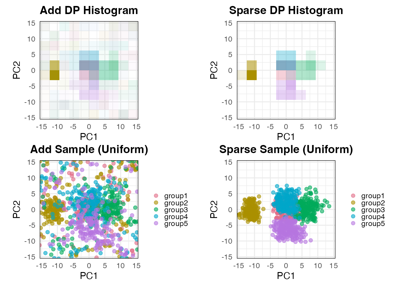

Group colors are assigned automatically according to the following rules:

• If all group labels are valid color names recognized by R (e.g., "red", "blue", and "green"), those colors are used directly.
• Otherwise, colors are automatically generated using the "Dark 3" palette from grDevices::hcl.colors().
• Users can override the automatic colors by specifying group_colors through score_plot_control().

For example, we can assign custom colors to the five groups and adjust the histogram transparency:

group_colors <- c(
  group1 = "#0072B2", group2 = "#D55E00", group3 = "#009E73",
  group4 = "#CC79A7", group5 = "#E69F00"
)

group_hist_plot <- plot(
  group_fit,
  sampling_control = sampling_control(
    method = "uniform", sample_size = 500
  ),
  plot_control = score_plot_control(
    group_colors = group_colors,
    hist_alpha_range = c(0, 0.75)
  )
)

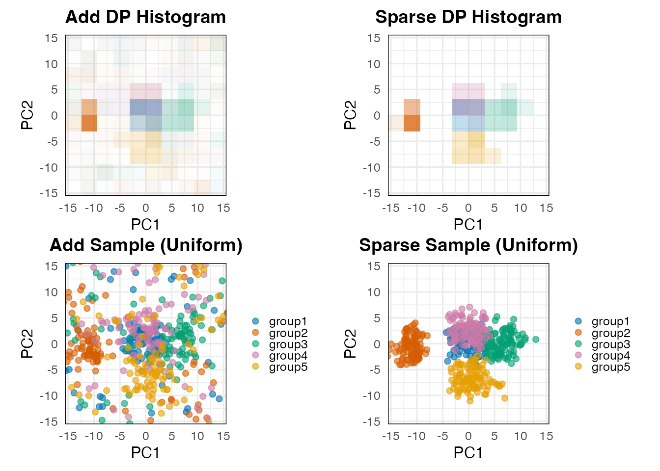
The hist_alpha_range argument controls the transparency range, with c(0, 0.75) setting the maximum opacity to 0.75. Each group’s bin probabilities are normalized within that group. Also, sample_size = 500 requests 500 points across all groups, not 500 per group.

For complete argument descriptions, see ?dp_score, ?plot.dp_score, ?score_plot_control, and ?sampling_control. For a combined scree, score, and loading analysis, continue to DP PCA Visualization.

---

Previous: DP Scree Plot
Next: DP PCA Visualization
Tutorial overview: Choose a starting point