DP PCA Visualization

What you will make

This tutorial uses the vowel dataset to create a grouped PCA analysis with dp_pca(). One fitted object supplies five displays:

Display	What it shows	A useful question
Scree/PVE	Estimated variation along the retained PC directions	How is the estimated variation distributed across components?
Score	A private histogram or synthetic points on two PC axes	How do the vowel groups overlap in this view?
Loading	Coefficients of the PC direction vectors	Which acoustic features contribute to the displayed directions?
Variable	Correlation-style variable coordinates	How strongly do the retained components represent each feature?
Biplot	Score points and variable arrows together	How do the displayed observations and features relate geometrically?

This tutorial focuses on R arguments, stored results, and plots. For the mathematics underlying all five displays, see DP PCA Visualization Methodology. The individual estimation mechanisms are covered by DP Directions Methodology, DP Scree Methodology, and DP Score Methodology. For general setup and input requirements, see Getting Started.

1. Load the vowel data

library(dppca)
data("vowel", package = "dppca")
X <- vowel

dim(X)
#> [1] 990  14
names(X)
#>  [1] "Split"   "Speaker" "Sex"     "F0"      "F1"      "F2"      "F3"     
#>  [8] "F4"      "F5"      "F6"      "F7"      "F8"      "F9"      "Class"

vowel contains 990 observations and 14 columns. For more details, see the documentation for vowel.

Columns	Contents	Role in this tutorial
`F0`–`F9`	Ten numeric acoustic features	PCA variables
`Split`	Training/test membership	Excluded categorical column
`Speaker`	Speaker identity, with 15 levels	Excluded categorical column
`Sex`	Speaker sex	Excluded categorical column
`Class`	Vowel category, with 11 levels	Group label, excluded from PCA variables

Keep X as a data frame. dp_pca() retains numeric features and reports the excluded columns. There is no need to manually remove the four categorical columns or convert them to numbers.

2. Create the privacy allocation

Integrated PCA needs three components: loading, scree, and score. When split is omitted, dp_pca() gives each stage one third of the total epsilon and delta:

privacy <- privacy_control(eps = 10, delta = 1e-4)
privacy$total
#>   eps delta 
#> 1e+01 1e-04
privacy$budgets
#> $loading
#>          eps        delta 
#> 3.333333e+00 3.333333e-05 
#> 
#> $scree
#>          eps        delta 
#> 3.333333e+00 3.333333e-05 
#> 
#> $score
#>          eps        delta 
#> 3.333333e+00 3.333333e-05

3. Fit DP PCA analysis

In dp_pca(), exactly one method must be selected for each estimation step:

Scree estimation: One of "clipped", "pmwm", or "huber". See the DP Scree Plot Tutorial for details.
Score histogram estimation: One of "add" or "sparse". See the DP Score Plot Tutorial for details.

Main arguments of `dp_pca()`

Argument	Description
`X`	Input data matrix or data frame with at least two numeric variables. Non-numeric columns are excluded from the PCA features.
`privacy`	Privacy settings from `privacy_control()`, allocated to loading, scree, and score estimation.
`scree`	Required list specifying `k`, `method`, `control`, and optionally `mono`. Defaults within the list are `k = NULL` (all components), `method = "clipped"`, and `mono = TRUE`; a method-specific `control` is required.
`score`	List specifying the private histogram `method` (`"sparse"` or `"add"`) and `bins`. Defaults: `method = "sparse"`, `bins = c(20, 20)`.
`axes`	Two distinct PC indices used for the score plot and biplot. Default: `c(1, 2)`.
`group`	Optional grouping column name or vector of group labels. The grouping column is excluded from PCA features. Default: `NULL`.
`non_private`	Whether to compute and store an ordinary PCA reference for comparison. If `TRUE`, `plot()` automatically displays both ordinary and DP results; if `FALSE`, only DP results are shown. Default: `FALSE`.
`V_dp`	Optional previously estimated full private PC direction matrix. When supplied, loading estimation is skipped. Default: `NULL`.
`cpp.option`	Whether to use the compiled implementation when estimating private PC directions internally. Default: `TRUE`.

For detailed explanations of the scree and score options, including available estimation methods and their tuning parameters, see the DP Scree Plot Tutorial and DP Score Plot Tutorial, respectively.

The V_dp argument allows previously estimated private PC directions to be reused in dp_score(). For a detailed example, see Reusing Private PC Directions in the DP Scree Plot tutorial.

Estimate four scree components and use PC1 and PC2 for the score grid:

set.seed(123)
pca_fit <- dp_pca(
  X,
  privacy = privacy,
  scree = list(
    k = 4,
    method = "clipped",
    control = clipped_control(C_clip = 3)
  ),
  score = list(method = "sparse", bins = c(9, 9)),
  axes = c(1, 2),
  group = "Class"
)
#> Warning: PCA: 10 numeric variables used.
#> Excluded from PCA (4): Split, Speaker, Sex, Class.
#> Grouping variable: Class
#> Groups (11): 0, 1, 2, 3, 4, 5, 6, 7, 8, 9, 10

pca_fit
#> Differentially Private PCA
#> Data: 990 observations x 10 variables
#> Components: 10 PC directions; 4 scree estimates
#> Score axes: PC1, PC2 
#> Group variable: Class 
#> Groups: 0, 1, 2, 3, 4, 5, 6, 7, 8, 9, 10 
#> Methods: scree = clipped ; score = sparse 
#> Total privacy budget: eps = 10 ; delta = 1e-04 
#> Non-private reference: not stored

The fit reports that ten numeric variables are used, that Split, Speaker, Sex, and Class are excluded from PCA, and that the grouping variable is Class. It also lists the 11 observed vowel groups.

4. Inspect the results

The summary reports estimated component importance, the allocated privacy budgets, selected axes, and group information.

pca_summary <- summary(pca_fit)
pca_summary
#> DP PCA Summary
#> Data: 990 observations x 10 variables
#> Components: 10 PC directions; 4 scree estimates
#> Score axes: PC1, PC2 
#> Methods: scree = clipped ; score = sparse 
#> Group variable: Class 
#> Groups: 0, 1, 2, 3, 4, 5, 6, 7, 8, 9, 10 
#> 
#> DP component importance:
#>                   PC1    PC2    PC3    PC4
#> Eigenvalue     1.3422 0.9141 0.6679 0.5366
#> PVE            0.3878 0.2641 0.1930 0.1551
#> Cumulative PVE 0.3878 0.6520 0.8449 1.0000
#> 
#> Proportions are normalized over 4 estimated components.
#> 
#> Allocated privacy budget:
#>                    eps     delta
#> Loading          3.333 3.333e-05
#> Scree            3.333 3.333e-05
#> Score frame      1.167 0.000e+00
#> Score histogram  2.167 3.333e-05
#> Total           10.000 1.000e-04
#> 
#> Non-private reference: not stored

Stored component	Contains
`pca_fit$directions`	The full 10-by-10 private direction matrix
`pca_fit$scree`, `$pve`	Four estimated scree values and their normalized contributions
`pca_fit$frame`, `$hist`	The private frame and pooled score histogram
`pca_fit$score_groups`	Private histograms for the vowel groups
`pca_fit$metadata$privacy$total`, `$budgets`	Total and stage-specific privacy budgets
`pca_fit$metadata$group_name`, `$group_levels`	The selected group name and observed group levels
`pca_fit$nonprivate`	The optional ordinary-PCA comparison results

pca_fit$metadata$privacy$total
#>   eps delta 
#> 1e+01 1e-04
pca_fit$metadata$privacy$budgets
#> $loading
#>          eps        delta 
#> 3.333333e+00 3.333333e-05 
#> 
#> $scree
#>          eps        delta 
#> 3.333333e+00 3.333333e-05 
#> 
#> $score
#>          eps        delta 
#> 3.333333e+00 3.333333e-05

5. Create all five displays

The shortest way to draw the five plots from an existing fit is:

plot(pca_fit)
#> Warning: The private histogram contains no positive probability mass; no
#> synthetic score points were generated.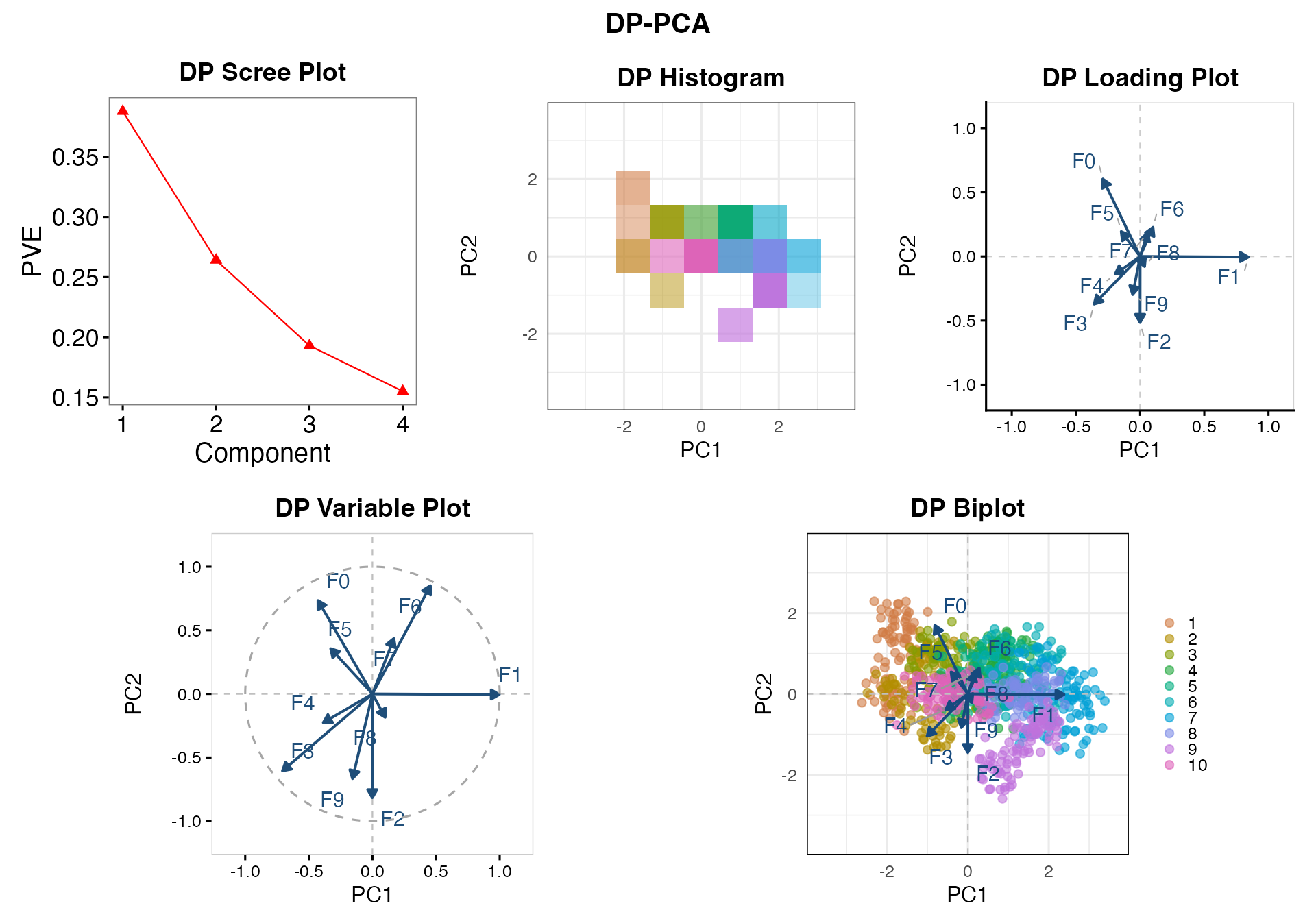

Result of DP-PCA

If fitted with non_private = TRUE, it automatically shows the ordinary reference page first, followed by the DP page.

set.seed(456)
pca_plots <- plot(
  pca_fit,
  display = "all",
  scree = list(
    type = "pve",                # "pve" or "scree"
    plot_control = NULL
  ),
  score = list(
    type = "sample",             # "histogram" (default) or "sample"
    plot_control = NULL
  ),
  loading = list(
    type = "vector",            # "vector" (default), "point", or "heatmap"
    heatmap_components = NULL,
    plot_control = NULL
  ),
  variable = list(
    plot_control = NULL         
  ),
  biplot = list(
    alpha = 0,
    labels = TRUE,
    plot_control = NULL
  ),
  sampling = sampling_control(  # Shared by score and biplot 
    method = "uniform",
    sample_size = NULL,
    bandwidth_scale = NULL
  ),
  center = TRUE,                # Shared by score and biplot 
  variables = 10,               # Shared by loading, variable and biplot 
  base_size = 12
)

Argument	Description
`display`	Selects which of the five PCA plots to display. Default: `"all"`.
`sampling`	Controls synthetic point sampling for the score sample plot and biplot.
`center`	Applies the same display-centering setting to the score plot and biplot. Default: `TRUE`.
`variables`	Selects variables displayed in the loading, variable, and biplot panels. Default: `10`.
`base_size`	Sets the base font size. Default: `12`.

The sampling argument controls how synthetic points are generated from the score histogram. The same sampled points are used in the score sample plot and biplot. See the DP Score Plot Tutorial for details.

By default, variables = 10 selects the 10 variables with the largest Euclidean norms of their private loading coefficients on the two selected PC axes. The same variables are displayed in the loading, variable, and biplot panels, including non-private comparisons. See the DP Loading Plot Tutorial for details on variable selection.

The center argument controls whether the DP score and biplot displays are shifted using the privately estimated score-frame midpoint. By default, center = TRUE places the private frame center at the origin and allows the biplot variable arrows to start at (0,0). See Display Centering for details.

For plot appearance, replace plot_control = NULL with a suitable control:

Scree: scree_plot_control(...). See the DP Scree Plot Tutorial.
Score: score_plot_control(...). See the DP Score Plot Tutorial.
Loading: loading_plot_control(...). See the DP Loading Plot Tutorial.
Variable and biplot: plot_control = list(...) for colors, arrow width, label size, and other display settings.

6. Reuse and export the results

The return value of plot(pca_fit) is a list, not a special plot class.

Component	Contains
`pca_plots$private$plots`	Named ggplot panels
`pca_plots$private$page`	The assembled page grob
`pca_plots$private$sampled_points`	Generated points before display centering and biplot scaling
`pca_plots$private$biplot`	Biplot coordinate and scaling metadata
`pca_plots$nonprivate`	The corresponding ordinary display components, when shown

# One figure
ggplot2::ggsave(
  "vowel-private-biplot.png",
  plot = pca_plots$private$plots$biplot,
  width = 7, height = 6, dpi = 300
)

# One complete saved page
grDevices::pdf("vowel-private-pca.pdf", width = 12, height = 8.5)
grid::grid.newpage()
grid::grid.draw(pca_plots$private$page)
grDevices::dev.off()

# The fit can be saved separately for a later R session.
saveRDS(pca_fit, "vowel-pca-fit.rds")

For complete argument descriptions, see ?dp_pca, ?plot.dp_pca, and ?sampling_control.

Previous: DP Score Plot
Tutorial overview: Choose a starting point