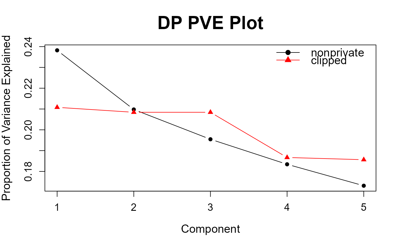
Plot differentially private scree estimates

This function computes and visualizes scree curves for principal component analysis, including the usual non-private curve and one or more differentially private estimates. It is a plotting wrapper around dp_scree() and returns a ggplot object.

Usage

dp_scree_plot(
  X,
  k,
  method = c("clipped", "pmwm", "huber"),
  control = NULL,
  eps,
  delta,
  center = TRUE,
  standardize = FALSE,
  g_dppca = FALSE,
  cpp.option = FALSE,
  mono = TRUE,
  type = c("pve", "scree")
)

Arguments

X: A numeric matrix or data frame. Rows correspond to observations and columns correspond to variables.
k: Positive integer defining the number of leading principal components to estimate. Must be an integer between 1 and the number of columns in X.
method: Scree estimation method or methods to plot. One or more of "clipped", "pmwm", or "huber". If omitted, "clipped" is used.
control: Optional method-specific control list, or a named list of control lists when multiple methods are requested. Use clipped_control(), pmwm_control(), and huber_control().
eps: Positive number defining the total epsilon privacy parameter. If g_dppca = TRUE, it is split between private direction estimation and private scree estimation.
delta: Number in (0, 1) defining the total delta privacy parameter. If g_dppca = TRUE, it is split between private direction estimation and private scree estimation.
center: A logical value indicating whether to center the columns of X before computing principal component directions. The default is TRUE.
standardize: A logical value indicating whether to scale the columns of X by their sample standard deviations after optional centering. The default is FALSE.
g_dppca: A logical value indicating whether to use private principal component directions for scree estimation. The default is FALSE. See dp_pc_dir() for details.
cpp.option: A logical value passed to dp_pc_dir() when g_dppca = TRUE. The default is FALSE. When g_dppca = TRUE, dp_pc_dir() is called with arguments eps = eps / 2 and delta = delta / 2.
mono: A logical value indicating whether to apply monotone post-processing to the private scree vector. The default is TRUE.
type: Quantity to plot. Use "pve" to plot proportions of variance explained and "scree" to plot raw scree values. The default is "pve".

Value

Invisibly returns a list with components:

nonprivate: non-private scree and PVE values.
results: method-specific dp_scree() outputs used in the plot.

Details

This function is a plotting wrapper around dp_scree(). For each requested method, it computes a private scree estimate and overlays it with the corresponding non-private curve. When type = "pve", the plotted quantity is the proportion of variance explained (PVE); when type = "scree", the raw scree values are shown.

To plot multiple methods, pass a character vector to method. If a method requires tuning parameters, pass control as a named list, for example control = list(clipped = clipped_control(), pmwm = pmwm_control(), huber = huber_control()).

For the estimating equations, privacy-budget allocation, and method-specific construction, see dp_scree().

References

Dwork C, Roth A (2014). “The Algorithmic Foundations of Differential Privacy.” Found. Trends Theor. Comput. Sci., 9(3–4), 211–407. ISSN 1551-305X, doi:10.1561/0400000042 .

Ramsay K, Spicker D (2025). “Improved subsample-and-aggregate via the private modified winsorized mean.” Code available at https://github.com/12ramsake/PMWM, 2501.14095, https://arxiv.org/abs/2501.14095.

Yu M, Ren Z, Zhou W (2024). “Gaussian differentially private robust mean estimation and inference.” Bernoulli, 30(4), 3059–3088.

Kim M, Jung S (2025). “Robust and Differentially Private Principal Component Analysis.” Statistical Analysis and Data Mining: An ASA Data Science Journal, 18(6), e70053. doi:10.1002/sam.70053 .

Examples

data(gau, package = "dppca")

# Use a small subset to keep the example fast.
X <- gau[1:200, ]

# Draw a private scree plot using the clipped mean method.
set.seed(123)
dp_scree_plot(
  X,
  k = 5,
  method = "clipped",
  control = clipped_control(C_clip = 3),
  eps = 3,
  delta = 1e-3
)


# Multiple scree methods can be overlaid by passing a vector to `method`
# and a named list to `control`, for example:
# dp_scree_plot(
#   X,
#   k = 5,
#   method = c("clipped", "pmwm", "huber"),
#   control = list(
#     clipped = clipped_control(C_clip = 3),
#     pmwm = pmwm_control(a = 0, b = 50, trim_const = 10, eta = 0.01),
#     huber = huber_control(k_min_m2 = -10, k_max_m2 = 10, m2_frac = 1 / 4)
#   ),
#   eps = 3,
#   delta = 1e-3
# )